Acknowledgements
This online tutorial is made possible through support from the National Science Foundation (NSF; grants IGE-1806874 and DUE-2417294), and the Department of Human Development and Family Studies (HDFS) at Penn State. If you find this tutorial helpful, consider citing or sharing:
- Chow, S-M., & Lee, J., Park, J. J., Kuruppumullage P. D., Hammel T., Hallquist, M. N., Nord, E. A., Oravecz, Z., Perry, H. L., Lesser, L. M., & Pearl, D. K. (2024). Personalized Education through Individualized Pathways and Resources to Adaptive Control Theory-Inspired Scientific Education (iPRACTISE): Proof-of-Concept Studies for Designing and Evaluating Personalized Education. Journal of Statistics and Data Science Education, 32(2). 174-187. DOI: 10.1080/26939169.2024.2302181
Data preparation
In this tutorial, we will go through some possible ways to check assumptions and screen for outliers in the context of multiple linear regression (MLR). We will start with loading the data.
Load the data: Intercountry life-cycle savings data
We are using LifeCycleSavings, one of the data sets in R. Typing in
?LifeCycleSavings, we see the following description about
the data set.
Description
Data on the savings ratio 1960–1970.
A data frame with 50 observations on 5 variables.
[1] sr: numeric aggregate personal savings
[2] pop15: numeric % of population under 15
[3] pop75: numeric % of population over 75
[4] dpi: numeric real per-capita disposable income
[5] ddpi: numeric % growth rate of dpi
Details
Under the life-cycle savings hypothesis as developed by Franco Modigliani, the savings ratio (aggregate personal saving divided by disposable income) is explained by per-capita disposable income, the percentage rate of change in per-capita disposable income, and two demographic variables: the percentage of population less than 15 years old and the percentage of the population over 75 years old. The data are averaged over the decade 1960–1970 to remove the business cycle or other short-term fluctuations.
#data(savings) #load the data for today's demo
#?LifeCycleSavings #also appears under this name. Has more detailed info.

#Note that read.table can be used to read in data
#files of different extensions

#What is going to happen if you use header=TRUE?
savings = read.table(file='savings.txt',sep=",",
                     na.strings="NA",
                     header=FALSE,
                     row.names=1
                     )
colnames(savings) =  c("sr","pop15", "pop75", "dpi", "ddpi")

savings[order(savings$sr),]
You should also feel comfortable reading in an external data set
using e.g., the read.table command. If you need a
refresher, check out some of the resources featured in , by going to
Intro to R \(\rightarrow\)
Data wrangling \(\rightarrow\) Base R \(\rightarrow\) Importing. The
two-minute, bite-sized tutorials by Anthony Damico are great, for
instance.
Assumption checking: model set-up
g = lm(sr ~ pop15+pop75+dpi+ddpi,savings)
resid = residuals(g) #Extract model residuals
fitted = fitted(g) #Extract fitted values of the DV (Yhat)
data = cbind(resid,fitted,g$model) #This data set contains the original variables as well as the residuals and Yhat
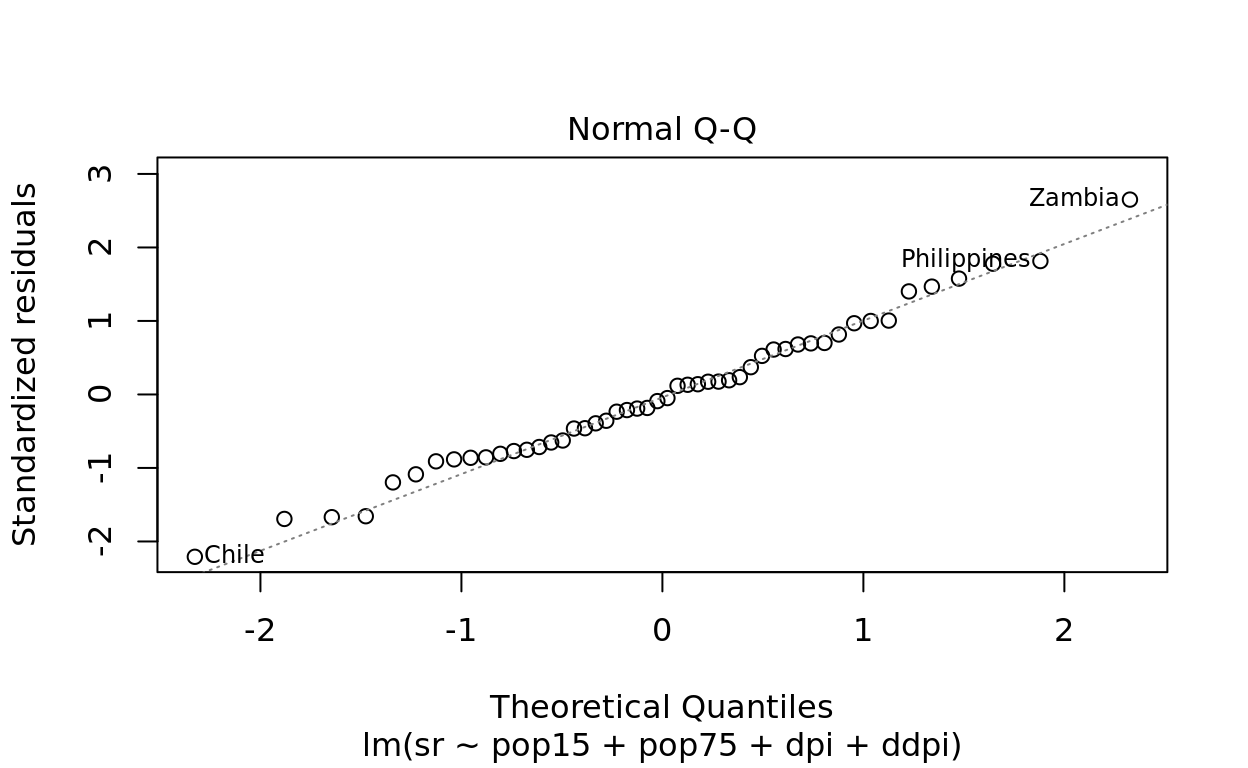
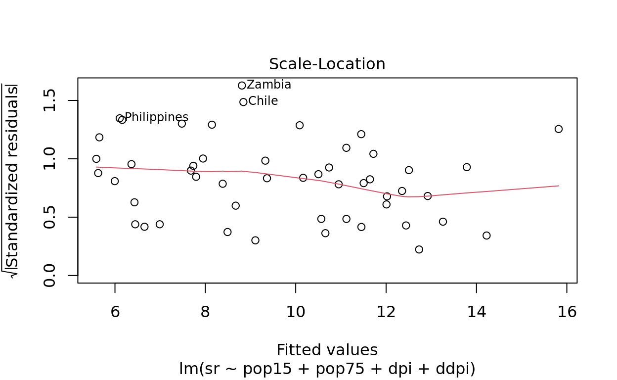
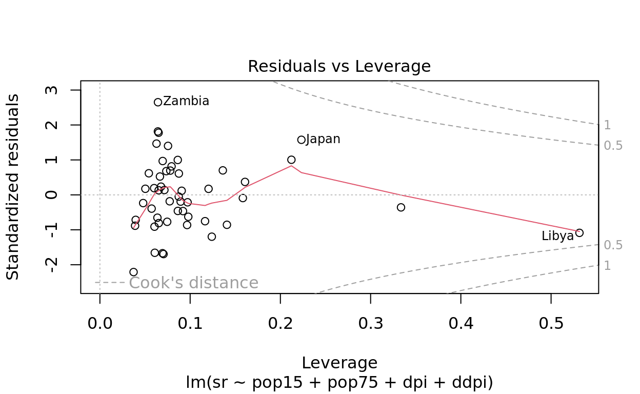
We are going to start by applying the “plot” function to the regression object to automatically generate 4 plots:
[1] plot of the residuals against Yhat
[2] QQplot of the standardized residuals (help screen for violation of normality assumption)
[3] Scale-location plot or S-L plot: plot of the square root of the absolute standardized residuals against Yhat
[4] Plot of the standardized residuals against leverage (a measure of the extremeness in IV values)
plot(g)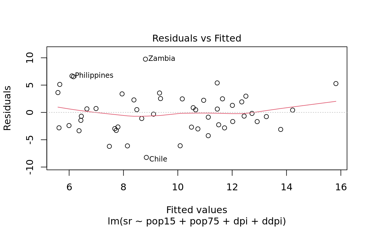
Omitted variables
One of the key assumptions in MLR is that all important independent variables (IVs) have been included in the regression model. Omission of important IVs leads to a misspecified model and may have serious consequences. For instance, the regression coefficients and the standard error estimates may both be biased.
We can create an added variable plot (AVP). The avPlot command from
the car library gives an easy way to do this, though it
requires that that the “added variable” (e.g., ddpi in this case) is
already included in the regression model g. Uncomment the
command avPlot below, put g in as the regression object,
and variable ddpi as the added variable to plot.
#avPlot(regressionObject, variable = "addedVariable")For more flexibility, create the plot ourselves. Here we write a function called plotSmooth that imposes Loess curve and least squares regression line in each plot.
plotSmooth <- function(data, mapping, ...){
  p <- ggplot(data = data, mapping = mapping) +
    geom_point() +
    geom_smooth(method=loess, fill="red", color="red", ...) +
    geom_smooth(method=lm, fill="blue", color="blue", ...)
  p
}
Let’s say we want to evaluate whether to add ddpi to a regression model without ddpi, i.e., only with IVs pop15, pop75, and dpi, then we can create such an AVP by:
# Specify g.IV as a model in which ddpi (the "added IV") is predicted using all other IVs
# g.IV = lm(ddpi ~ ?, data = savings)

# Get the residuals
# resid_ddpi = residuals(g.IV)

# Now specify g.DVnoddpi as a model in which the DV (sr) is predicted using all other IVs but ddpi
# g.DVnoddpi = lm(sr ~ ?, data=savings)

# Get the residuals from the model with no ddpi
# residsr_noddpi = residuals(g.DVnoddpi)
Now we can call our plotSmooth function above - basically we want to see if there is any systematic relation between the added variable (ddpi) and the residuals of sr - after trying to explain it using all remaining IVs.
plotSmooth(data.frame(residIV = resid_ddpi, residy = residsr_noddpi),
           aes(residIV,residy))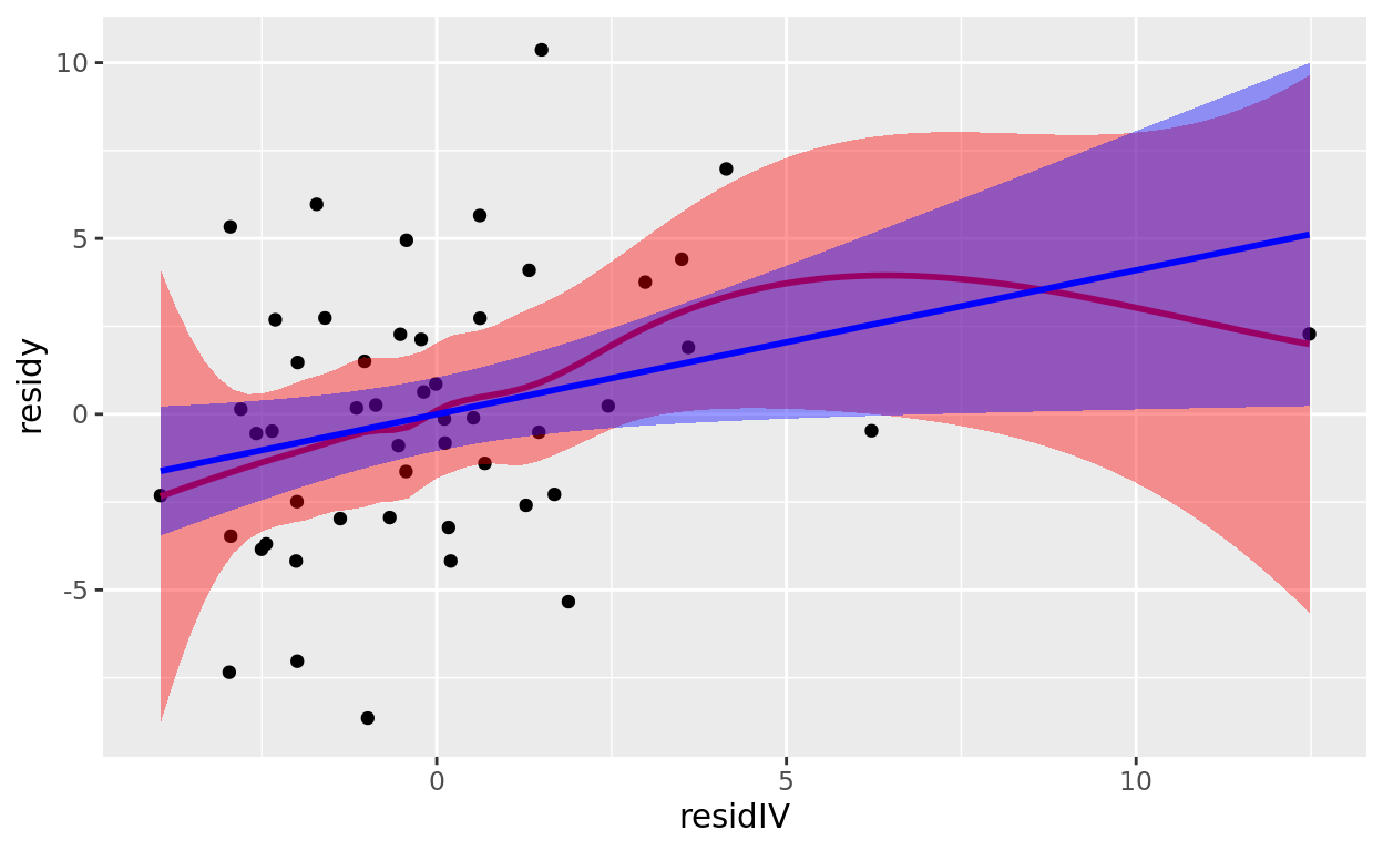
Remedy for omitted variables:
- Include the omitted variables
- When deciding whether a certain IV should be included, the decision
is simplest when theory and data are consistent with each other:
- Theory supports, AVP supports \(\rightarrow\) Include
- Theory and AVP do not support \(\rightarrow\) Do not include
- Ambiguous? Consider sensitivity analysis – check whether results involving other IVs change when you add (omit) a new IV to (from) the model.
Nonlinearity
Our MLR above assume linear relationships among the IVs and DV. If any of these relationships are severely nonlinear, estimates of regression coefficients and standard errors will be biased. Here we some some plots to help diagnose nonlinearity.
#Plot residuals against Yhat
plot(fitted,resid,xlab="Fitted",ylab="Residuals")
abline(h=0)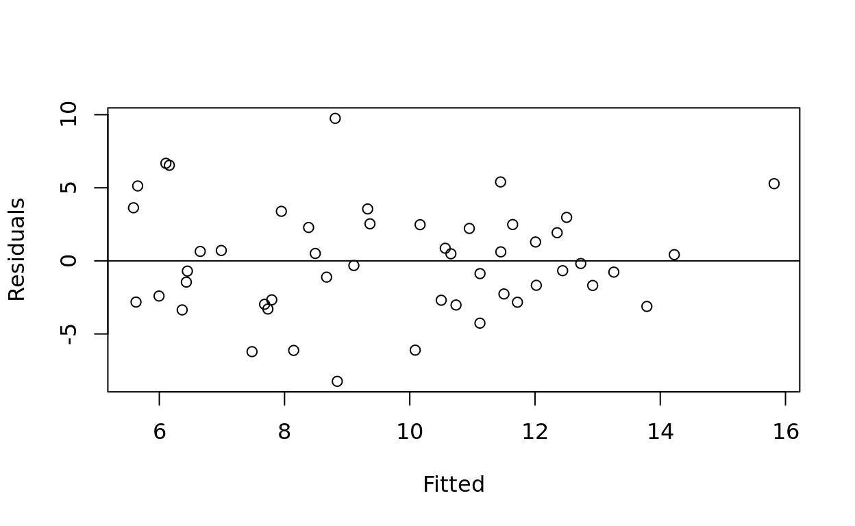
#Matrix scatterplot of everything
pairs(data,panel=panel.smooth)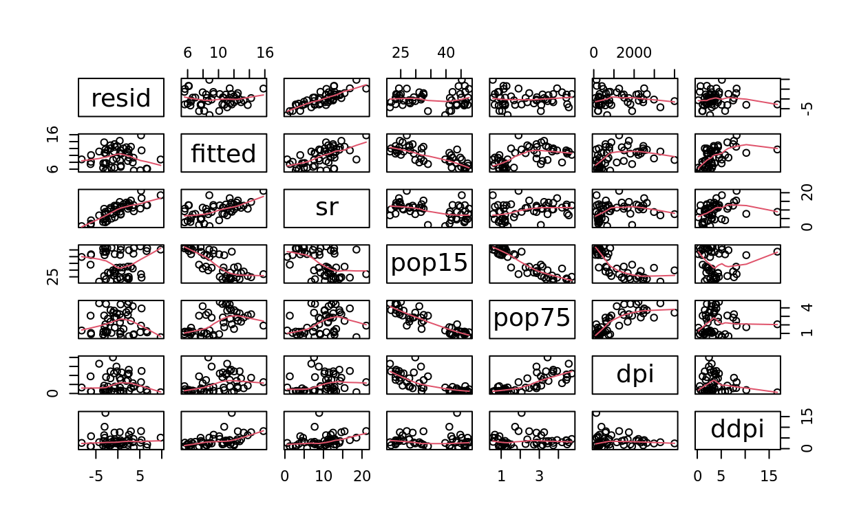
Here, in examining the plot of residuals against fitted (predicted \(y\)) values, we mostly want to see a flat straight line. Any systematic curvatures or deviations from a flat straight line may suggest the presence of nonlinear relations among variables.
We can also create a fancier-looking matrix scatter plot function building on ggpairs (requires GGally and ggplot2).
#pp = ggpairs(data,columns=c(4:7,2,3,1),
#             lower = list(continuous = plotSmooth))+
#  ggtitle('Original model')
#print(pp)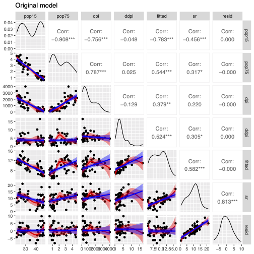
In the matrix scatterplot produced by ggpairs, let’s focus on the last row, which includes plots of residuals against each of the IVs, and also the fitted values (columns 1-5). We see mostly flat straight lines for the most part, except that in the ddpi column, the loess curve and its confidence interval (the red shaded region) do show slight deviations from a flat line. But this may be due more to outliers.
Homoscedastic variance of residuals
From the earlier plots and evaluation of (V1), we saw that there may be heteroscedasdicity in residuals related to pop15. That is, it looks like there is greater spread in residuals at pop15 \(>\) 35 than pop15 \(<\) 35 (see last row, first column of matrix scatter plot). Let’s take a closer look.
plotSmooth(data, aes(pop15,resid))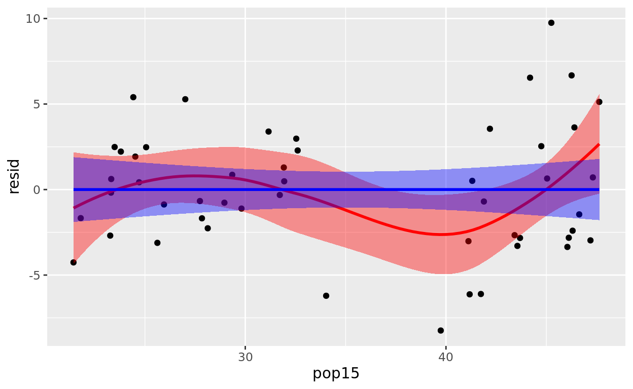
The variance looks larger for countries with pop15 >= 35. Let’s test this formally. Test for equality of variance between countries with pop15 > 35 and those with pop15 < 35.
var.test(residuals(g)[data$pop15 >= 35],residuals(g)[data$pop15 < 35], alternative = "two.sided")##
## F test to compare two variances
##
## data: residuals(g)[data$pop15 >= 35] and residuals(g)[data$pop15 < 35]
## F = 2.7851, num df = 22, denom df = 26, p-value = 0.01358
## alternative hypothesis: true ratio of variances is not equal to 1
## 95 percent confidence interval:
## 1.240967 6.430238
## sample estimates:
## ratio of variances
## 2.785067Oops. It looks like there is significant difference between the variances of the two groups.
An alternative to the F-test is the Levene’s test, which is more
robust to deviations from normality. To do this, let’s create a
variable, group, whose value indicates countries with pop15
\(\ge\) 35 (group = 0) vs. not (group =
1).
temp = data.frame(resid=residuals(g),group=factor(ifelse(data$pop15>=35,0,1)))
leveneTest(resid ~ group, data=temp, center=mean) #Alternative is center=median
var(residuals(g)[data$pop15 > 35])/var(residuals(g)[data$pop15 < 35]) #ratio of the two groups' variances## [1] 2.785067The Levene’s test also suggests significant heteroscedasdicity in variance. That said, the larger variance is about 2.79 times larger than the smaller variance – not too bad. Let’s do another check. Let’s divide pop15 into 10 bins or categories, and see if the ratio between the largest variance and the smallest variance is greater than 10.
data$pop15bin = quantileCut(data$pop15,10) #Create pop15bin, categories of pop15 based on quantile cuts

temp0 = group_by(data,pop15bin) #Group data by the 10 bins we have created via quantileCut
summarize(temp0,varResid=var(resid)) #Get residual variance by bin
#You can also accomplish the above by using the pipe operator, |>|, if you don't want
#to create the intermediate output, temp0.
data |>
group_by(pop15bin) |>
summarize(varResid = var(resid))Alright. So the ratio of the largest variance (38.1) to the smallest variance (1.4) is 38.1/1.4 = 27.21. In this example, much of the heterogeneity in residuals may stem from outliers though. Removal of outliers may help fix the issue.
Normality of residuals
Let’s check the normality of the residuals. In the code below, replace XXX with “residuals(regressionObject).”
#qqnorm(XXX,ylab="Residuals")
#qqline(XXX)


#qqPlot function from the car library
#qqPlot(XXX, main="qqPlot function from car")

#Use the Shapiro-Wilk test to check
#shapiro.test(XXX) #No significant deviations from normality
Oh good. We didn’t find evidence for significant deviations from normality in the residuals.
Remedy: Transformations of variables
This is likely an overkill for these data, as we did not have clear violations of the normality assumption. But let’s try it out anyway.
We are going to try finding the “optimal” box-cox transformation as follows.
bc = boxcox(g, lambda = seq(-2, 10, 1))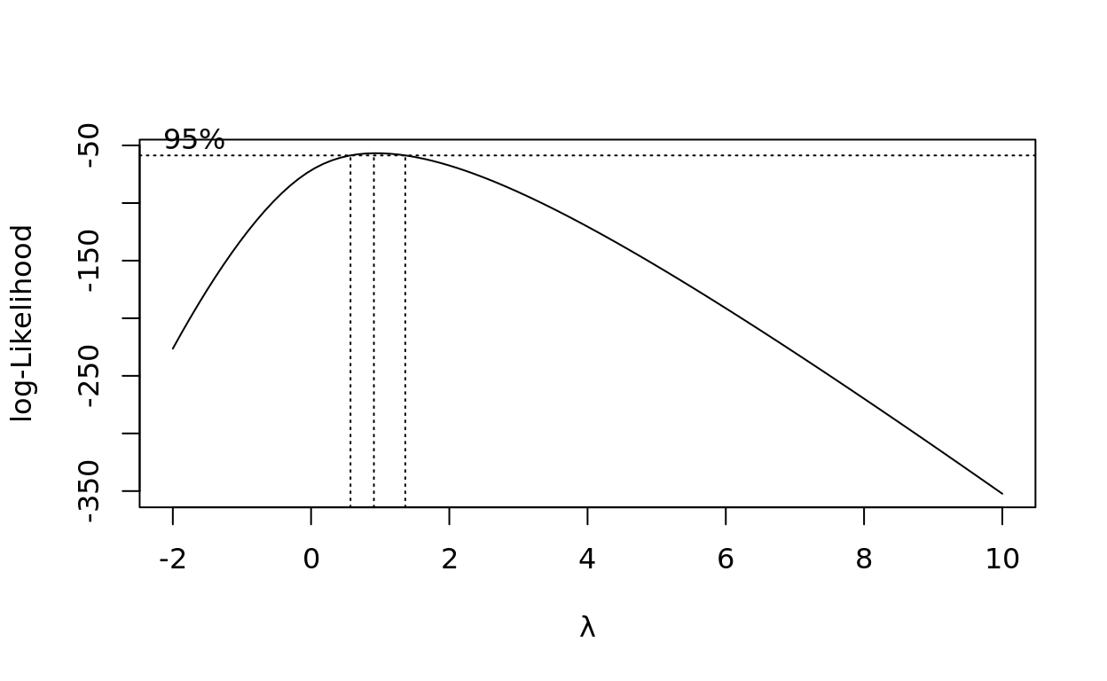
trans = bc$x[which.max(bc$y)] #Extract the power that maximizes the likelihood
#trans is basically close to 1. So transformation is not really needed in this case.
#But if you want to do it, this is how you would use the power in the lm:
g3 = lm(sr^trans ~ pop15+pop75+dpi+ddpi,savings)
data3 = data.frame(resid=residuals(g3),g3$model) #data3 has the new residuals and original variables

pp3 = plotSmooth(data3,aes(pop15,resid))+ ylim(-5,5)
print(pp3)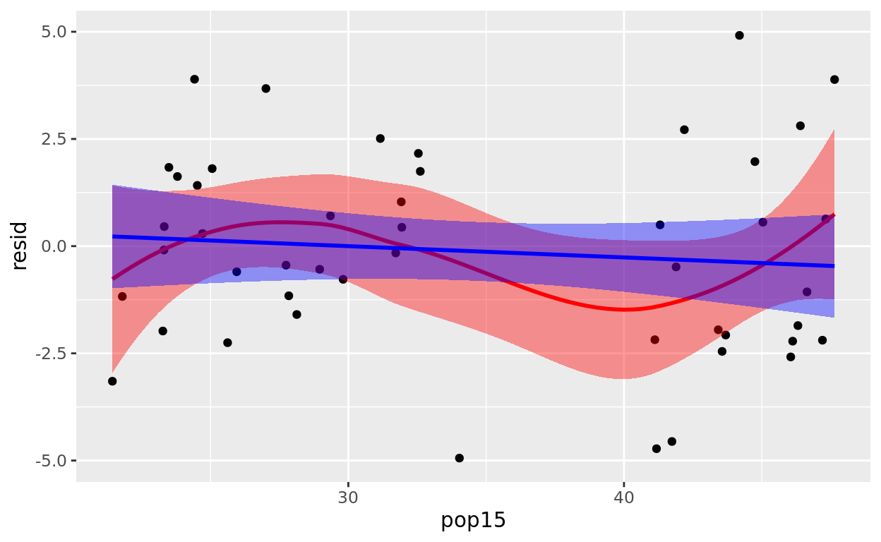
The boxcox function above suggests that a transformation to a power of 0.9 might help. We saw that this transformation is indeed helpful. That is, notice that the range of the residuals is slight reduced – if we use the same exact ylim as before, all the residuals would be more narrowly cluttered close to the flat line. However, it may be hard to explain what a power of 0.9 mean, and the 95% confidence intervals for the optimal power includes 1.0 (i.e., no transformation needed). So we likely don’t need to transform anything in this case.
Outlier and Colinearity Detection
Variance Inflation Factors
vif(g)## pop15 pop75 dpi ddpi
## 5.937661 6.629105 2.884369 1.074309The variance inflation factor quantifies the factor increase of the variance of \(B_j\) due to the linear dependence of \(x_j\) with the other IVs. VIF \(>\) 10 is usually regarded as problematic. VIF does not seem to be problematic in this data set.
Leverage
lev = hatvalues(g) #Get leverage

length(lev[lev <=0.000]) #Leverage values that are exactly 0 usually correspond to missing cases, or cases with values exactly equal to the means of the IVs (unlikely). Here we don't have any such cases because they have been omitted from the MLR
## [1] 0sum(lev) ## [1] 5n=dim(g$model)[1]
k=length(coef(g))-1 #No of IVs
k## [1] 4Here we see that the leverage values sum to the number of parameters = 5 (4 reg coefs + 1 intercept).
#If you are interested in how this comes about:
X = model.matrix(g)
H = X %*% solve(t(X)%*%X) %*% t(X) #This yields the n x n "hat" matrix
Hdiag = diag(H) #length = 50; one leverage value for each country in the data

head(lev)
## Australia Austria Belgium Bolivia Brazil Canada
## 0.06771343 0.12038393 0.08748248 0.08947114 0.06955944 0.15840239head(Hdiag)## Australia Austria Belgium Bolivia Brazil Canada
## 0.06771343 0.12038393 0.08748248 0.08947114 0.06955944 0.15840239The leverage values obtained using the command
hatvalues(.) match those computed manually, stored in
Hdiag.
#More extreme threshold
lev[lev>3*(k+1)/n]
## United States Libya
## 0.3336880 0.5314568#United States Libya
#0.3336880 0.5314568
#Less extreme threshold
lev[lev>2*(k+1)/n]## Ireland Japan United States Libya
## 0.2122363 0.2233099 0.3336880 0.5314568#Ireland Japan United States Libya
#0.2122363 0.2233099 0.3336880 0.5314568 Using the more extreme threshold (3*(k+1)/n), only two countries, United States and Libya, were found to have extreme leverage values. Using the less extreme threshold (2*(k+1)/n), Japan and Ireland were also found to be extreme in leverage.
Discrepancy: Studentized residual
rr=rstudent(g)

plot(rr,ylab="Studentized residuals")
abline(h=c(-2,2),col="red",lty=2)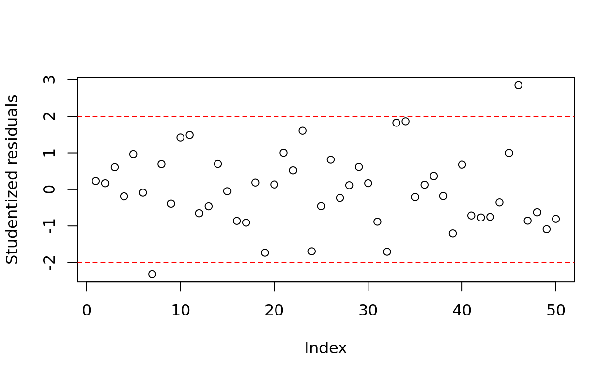
rr[abs(rr)>2]## Chile Zambia
## -2.313429 2.853558#Plot of square-root of standardized residuals
plot(g,which=3) # Zambia, Chile, Phillippines - based on studentized residuals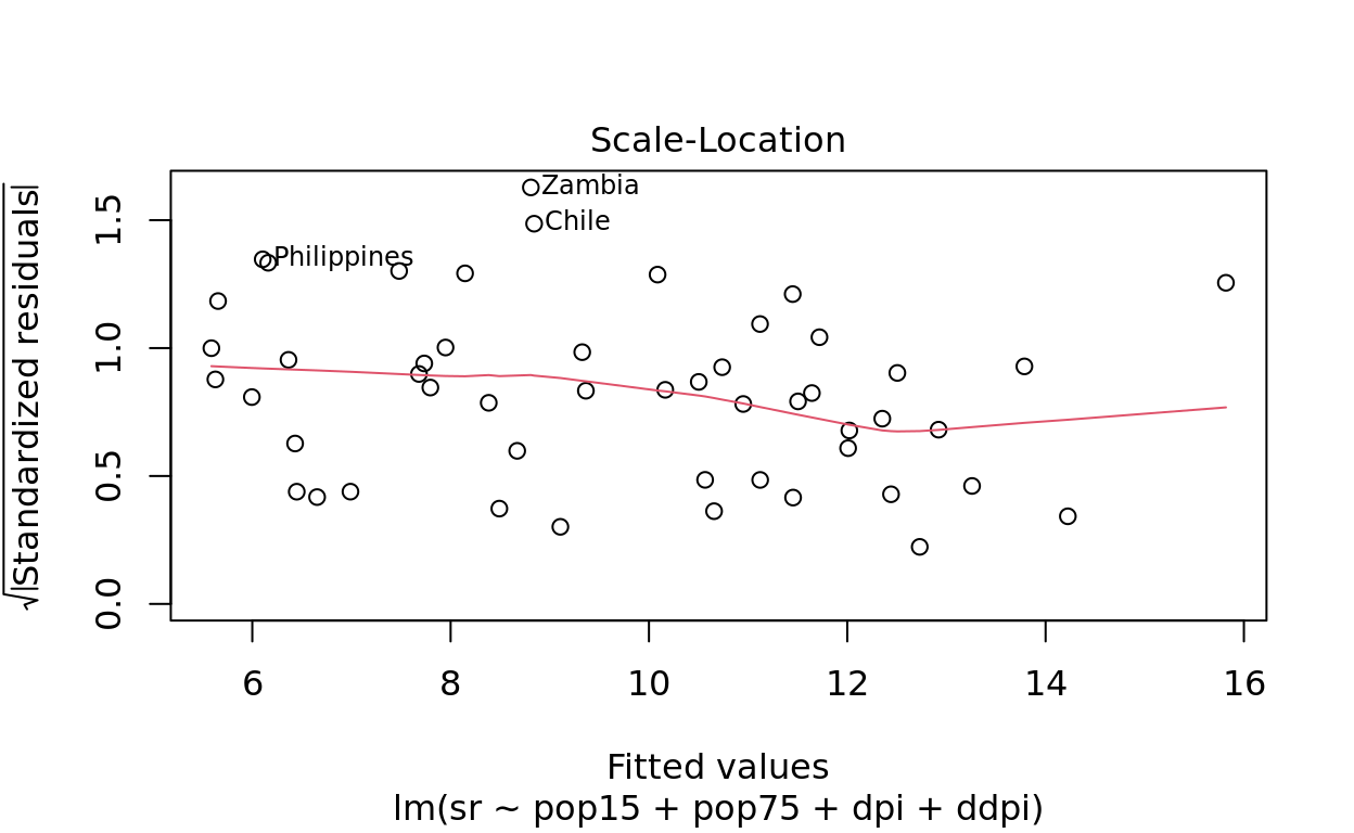
#Plot of standardized residuals against leverage
plot(g,which=5) #Zambia, Japan, Libya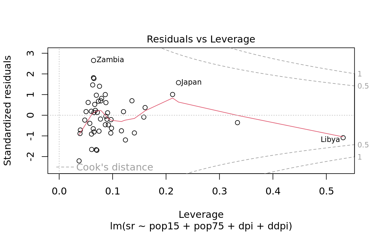
Chile, Zambia (all plots), and Phillippines (second plot) were found to be high in discrepancy. Japan, Libya are highlighted in the last plot more in terms of extreme leverage.
Global influence measures
dff = dffits(g)
plot(dff,ylab="DFFITS")
abline(h=c(-1,1)*2/sqrt(n),col="red",lty=2) 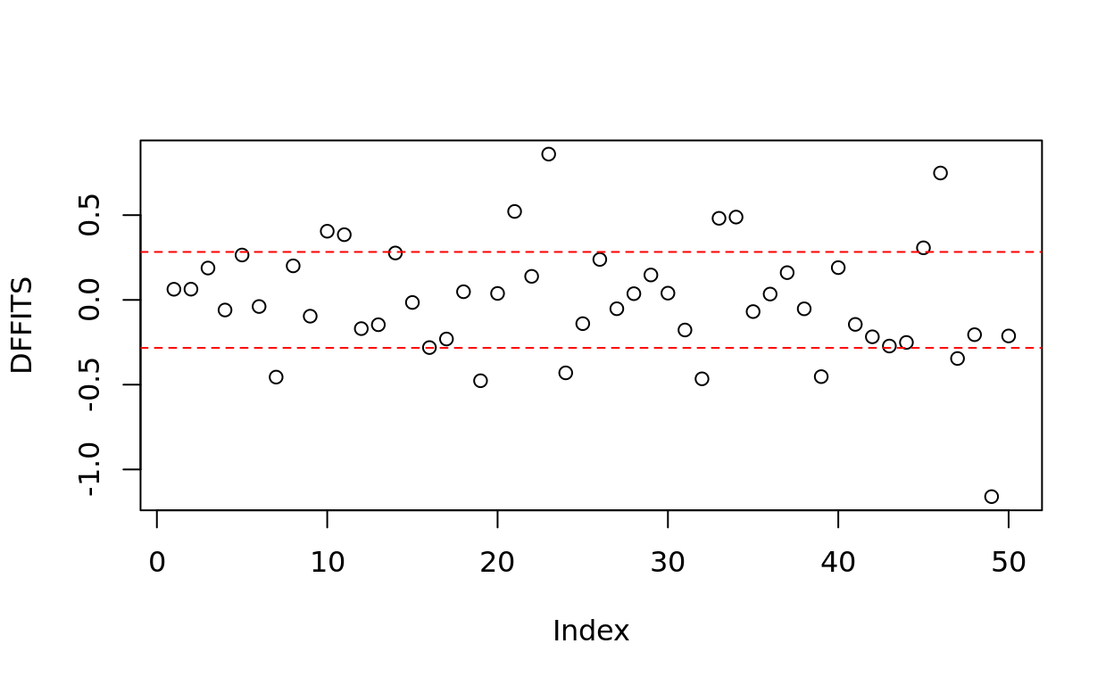
Perhaps too many countries were identified to be influential based on dffits.
cook=cooks.distance(g)
DCutoff = 2*sqrt((k+1)/n)
(DCutoff)
## [1] 0.6324555cook[cook > DCutoff] ## named numeric(0)plot(g,which=4) #Cook's d by observation number. Zambia, Libya, Japan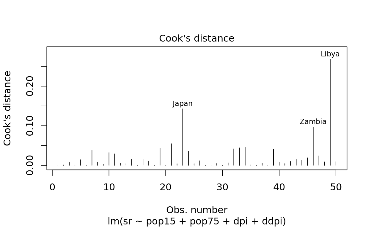
plot(g,which=6) #Cook's d against leverage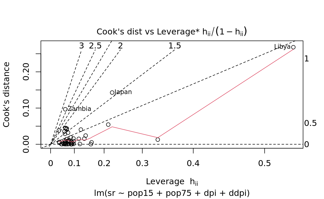
Using the threshold Dcutoff = 2\(\sqrt{(k+1)/n}\) \(=\) 0.63, none exceeded the threshold. However, Libya is identified as relatively influential based on Cook’s distance, and high in leverage.
Local influence measure: dfbeta
dfb = dfbetas(g)
#Thresholds: +/- 1 for small to moderate n; +-2/sqrt(n) for large n
r = rownames(dfb)
apply(dfb,2,function(x){r[abs(x)>1]})
## $`(Intercept)`
## character(0)
##
## $pop15
## character(0)
##
## $pop75
## character(0)
##
## $dpi
## character(0)
##
## $ddpi
## [1] "Libya"dfbetaPlots(g) #None exceeded the default small/moderate n threshold of +/- 1,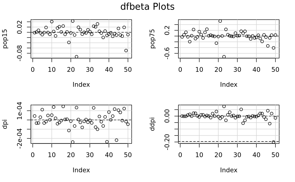
               #but closer inspection of the dfbetas indicated that Libya's dfbeta is
               #just above the threshold.
The function dfbetas(.) returns matrix of 50 \(\times\) 5 values for the 5 regression
parameters, including the intercept. Applying the threshold, \(\pm\) 1 for small to moderate n (use \(\frac{\pm 2}{\sqrt{n}}\) for large n),
Libya was found to be influential in affecting the regression
coefficient for ddpi, as was shown in the plot produced by
dfbetaPlots(.).
influence.measures and influencePlot
a = influence.measures(g)
a
## Influence measures of
## lm(formula = sr ~ pop15 + pop75 + dpi + ddpi, data = savings) :
##
## dfb.1_ dfb.pp15 dfb.pp75 dfb.dpi dfb.ddpi dffit cov.r
## Australia 0.01232 -0.01044 -0.02653 0.04534 -0.000159 0.0627 1.193
## Austria -0.01005 0.00594 0.04084 -0.03672 -0.008182 0.0632 1.268
## Belgium -0.06416 0.05150 0.12070 -0.03472 -0.007265 0.1878 1.176
## Bolivia 0.00578 -0.01270 -0.02253 0.03185 0.040642 -0.0597 1.224
## Brazil 0.08973 -0.06163 -0.17907 0.11997 0.068457 0.2646 1.082
## Canada 0.00541 -0.00675 0.01021 -0.03531 -0.002649 -0.0390 1.328
## Chile -0.19941 0.13265 0.21979 -0.01998 0.120007 -0.4554 0.655
## China 0.02112 -0.00573 -0.08311 0.05180 0.110627 0.2008 1.150
## Colombia 0.03910 -0.05226 -0.02464 0.00168 0.009084 -0.0960 1.167
## Costa Rica -0.23367 0.28428 0.14243 0.05638 -0.032824 0.4049 0.968
## Denmark -0.04051 0.02093 0.04653 0.15220 0.048854 0.3845 0.934
## Ecuador 0.07176 -0.09524 -0.06067 0.01950 0.047786 -0.1695 1.139
## Finland -0.11350 0.11133 0.11695 -0.04364 -0.017132 -0.1464 1.203
## France -0.16600 0.14705 0.21900 -0.02942 0.023952 0.2765 1.226
## Germany -0.00802 0.00822 0.00835 -0.00697 -0.000293 -0.0152 1.226
## Greece -0.14820 0.16394 0.02861 0.15713 -0.059599 -0.2811 1.140
## Guatamala 0.01552 -0.05485 0.00614 0.00585 0.097217 -0.2305 1.085
## Honduras -0.00226 0.00984 -0.01020 0.00812 -0.001887 0.0482 1.186
## Iceland 0.24789 -0.27355 -0.23265 -0.12555 0.184698 -0.4768 0.866
## India 0.02105 -0.01577 -0.01439 -0.01374 -0.018958 0.0381 1.202
## Ireland -0.31001 0.29624 0.48156 -0.25733 -0.093317 0.5216 1.268
## Italy 0.06619 -0.07097 0.00307 -0.06999 -0.028648 0.1388 1.162
## Japan 0.63987 -0.65614 -0.67390 0.14610 0.388603 0.8597 1.085
## Korea -0.16897 0.13509 0.21895 0.00511 -0.169492 -0.4303 0.870
## Luxembourg -0.06827 0.06888 0.04380 -0.02797 0.049134 -0.1401 1.196
## Malta 0.03652 -0.04876 0.00791 -0.08659 0.153014 0.2386 1.128
## Norway 0.00222 -0.00035 -0.00611 -0.01594 -0.001462 -0.0522 1.168
## Netherlands 0.01395 -0.01674 -0.01186 0.00433 0.022591 0.0366 1.229
## New Zealand -0.06002 0.06510 0.09412 -0.02638 -0.064740 0.1469 1.134
## Nicaragua -0.01209 0.01790 0.00972 -0.00474 -0.010467 0.0397 1.174
## Panama 0.02828 -0.05334 0.01446 -0.03467 -0.007889 -0.1775 1.067
## Paraguay -0.23227 0.16416 0.15826 0.14361 0.270478 -0.4655 0.873
## Peru -0.07182 0.14669 0.09148 -0.08585 -0.287184 0.4811 0.831
## Philippines -0.15707 0.22681 0.15743 -0.11140 -0.170674 0.4884 0.818
## Portugal -0.02140 0.02551 -0.00380 0.03991 -0.028011 -0.0690 1.233
## South Africa 0.02218 -0.02030 -0.00672 -0.02049 -0.016326 0.0343 1.195
## South Rhodesia 0.14390 -0.13472 -0.09245 -0.06956 -0.057920 0.1607 1.313
## Spain -0.03035 0.03131 0.00394 0.03512 0.005340 -0.0526 1.208
## Sweden 0.10098 -0.08162 -0.06166 -0.25528 -0.013316 -0.4526 1.086
## Switzerland 0.04323 -0.04649 -0.04364 0.09093 -0.018828 0.1903 1.147
## Turkey -0.01092 -0.01198 0.02645 0.00161 0.025138 -0.1445 1.100
## Tunisia 0.07377 -0.10500 -0.07727 0.04439 0.103058 -0.2177 1.131
## United Kingdom 0.04671 -0.03584 -0.17129 0.12554 0.100314 -0.2722 1.189
## United States 0.06910 -0.07289 0.03745 -0.23312 -0.032729 -0.2510 1.655
## Venezuela -0.05083 0.10080 -0.03366 0.11366 -0.124486 0.3071 1.095
## Zambia 0.16361 -0.07917 -0.33899 0.09406 0.228232 0.7482 0.512
## Jamaica 0.10958 -0.10022 -0.05722 -0.00703 -0.295461 -0.3456 1.200
## Uruguay -0.13403 0.12880 0.02953 0.13132 0.099591 -0.2051 1.187
## Libya 0.55074 -0.48324 -0.37974 -0.01937 -1.024477 -1.1601 2.091
## Malaysia 0.03684 -0.06113 0.03235 -0.04956 -0.072294 -0.2126 1.113
## cook.d hat inf
## Australia 8.04e-04 0.0677
## Austria 8.18e-04 0.1204
## Belgium 7.15e-03 0.0875
## Bolivia 7.28e-04 0.0895
## Brazil 1.40e-02 0.0696
## Canada 3.11e-04 0.1584
## Chile 3.78e-02 0.0373 *
## China 8.16e-03 0.0780
## Colombia 1.88e-03 0.0573
## Costa Rica 3.21e-02 0.0755
## Denmark 2.88e-02 0.0627
## Ecuador 5.82e-03 0.0637
## Finland 4.36e-03 0.0920
## France 1.55e-02 0.1362
## Germany 4.74e-05 0.0874
## Greece 1.59e-02 0.0966
## Guatamala 1.07e-02 0.0605
## Honduras 4.74e-04 0.0601
## Iceland 4.35e-02 0.0705
## India 2.97e-04 0.0715
## Ireland 5.44e-02 0.2122
## Italy 3.92e-03 0.0665
## Japan 1.43e-01 0.2233
## Korea 3.56e-02 0.0608
## Luxembourg 3.99e-03 0.0863
## Malta 1.15e-02 0.0794
## Norway 5.56e-04 0.0479
## Netherlands 2.74e-04 0.0906
## New Zealand 4.38e-03 0.0542
## Nicaragua 3.23e-04 0.0504
## Panama 6.33e-03 0.0390
## Paraguay 4.16e-02 0.0694
## Peru 4.40e-02 0.0650
## Philippines 4.52e-02 0.0643
## Portugal 9.73e-04 0.0971
## South Africa 2.41e-04 0.0651
## South Rhodesia 5.27e-03 0.1608
## Spain 5.66e-04 0.0773
## Sweden 4.06e-02 0.1240
## Switzerland 7.33e-03 0.0736
## Turkey 4.22e-03 0.0396
## Tunisia 9.56e-03 0.0746
## United Kingdom 1.50e-02 0.1165
## United States 1.28e-02 0.3337 *
## Venezuela 1.89e-02 0.0863
## Zambia 9.66e-02 0.0643 *
## Jamaica 2.40e-02 0.1408
## Uruguay 8.53e-03 0.0979
## Libya 2.68e-01 0.5315 *
## Malaysia 9.11e-03 0.0652influencePlot(g) 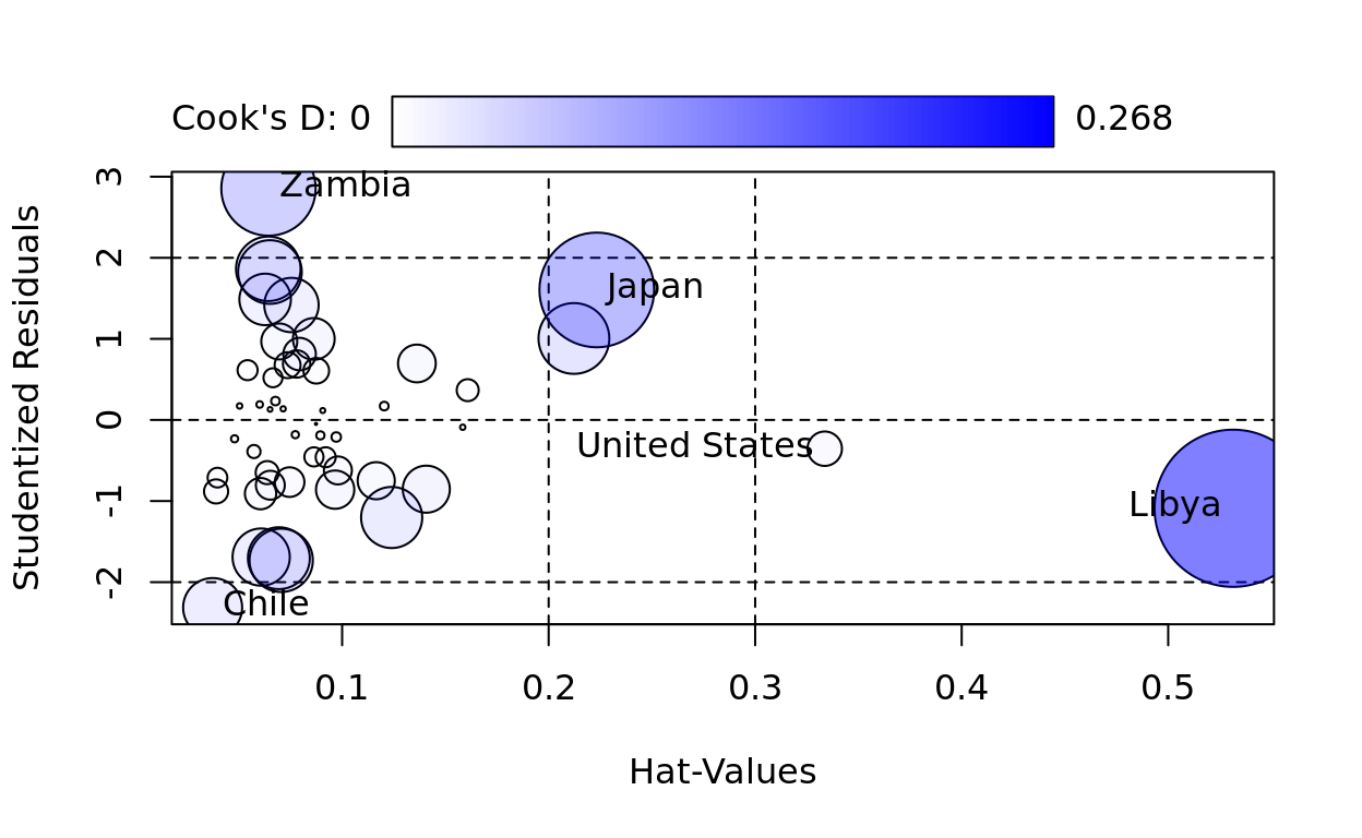
Influence.measures is a “one-stop” command that produces a bunch of diagnostic measures, including dfbetas, cook’s distance, and leverage (“hat”). Cases which are influential with respect to any of the printed measures are marked with an asterisk.
The command influencePlot(.) creates a “bubble” plot of
Studentized residuals by leverage values, with the areas of the circles
proportional to the cases’ Cook’s ds.
Zambia and Chile are extreme in terms of discrepancy (value of \(y\)). Libya is relatively large in leverage (predictor values), dfbeta value for ddpi, and Cook’s distance, but its cook’s distance hasn’t exceeded the threshold.
Remedy: Outlier removal
We can identify individual cases quickly with the “identify” function
plot(data$ddpi, data$resid)
identify(x=data$ddpi, y=data$resid, label=rownames(data)) 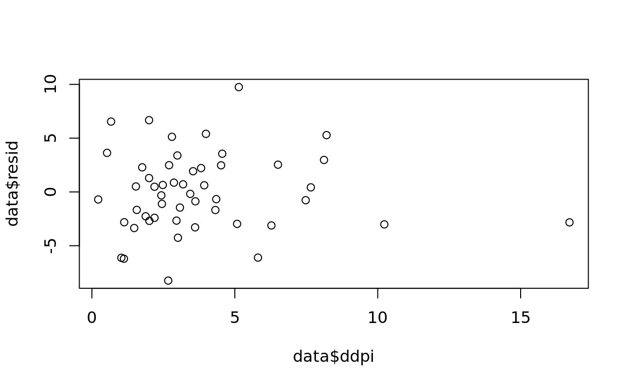
## integer(0)rownames(data)[c(46,49)]## [1] "Zambia" "Libya"#Libya, Zambia as potential "outliers" - influence in a future class
plot(data$pop15, data$resid)
identify(x=data$pop15, y=data$resid, label=rownames(data)) #Zambia as potential "outlier"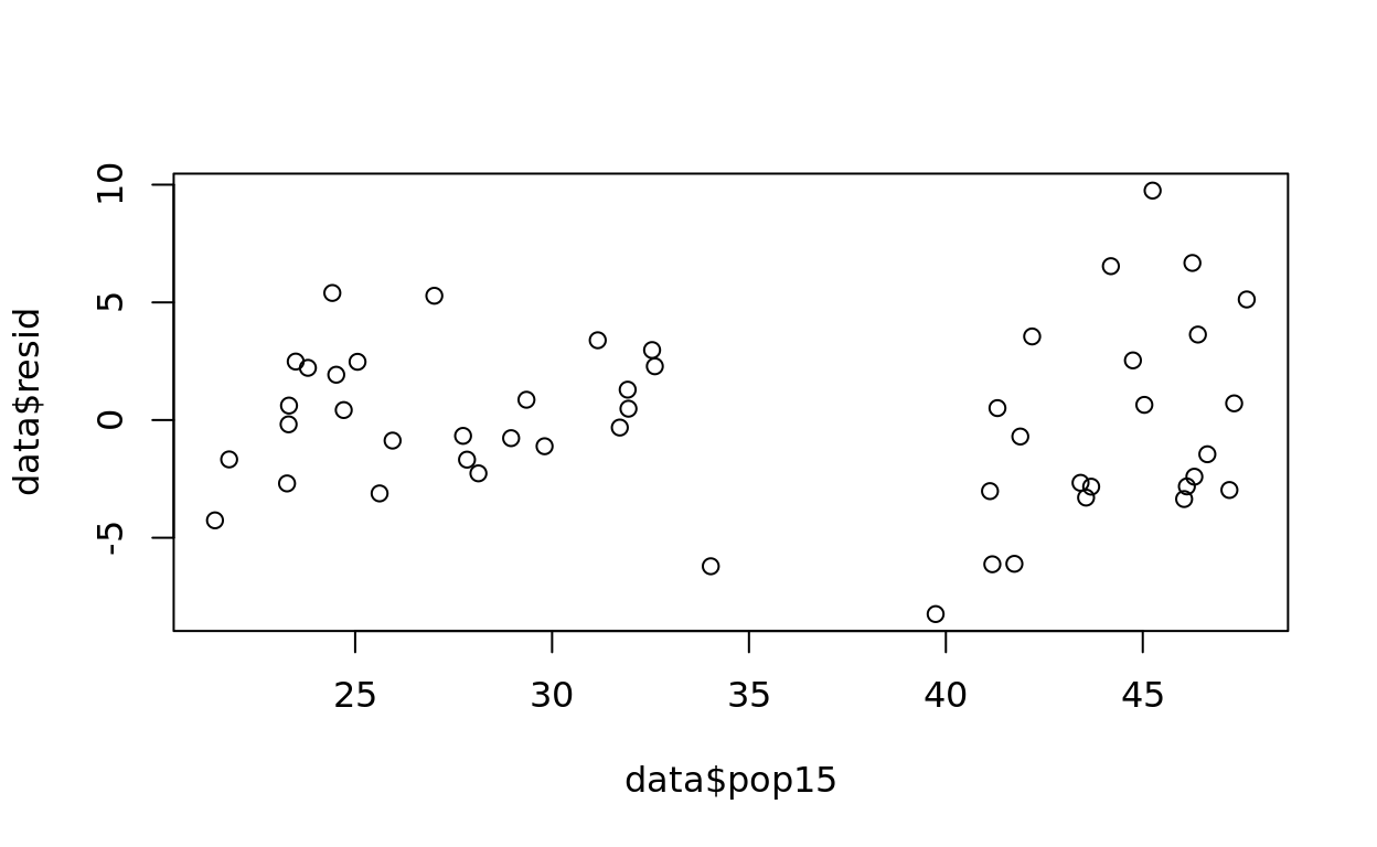
## integer(0)We are going to try removing Zambia, Libya, and Chile from our analysis.
savings2 = savings[!rownames(savings) %in% c("Zambia","Libya", "Chile"),]
g4 = lm(sr ~ pop15+pop75+dpi+ddpi,savings2)
summary(g4)
##
## Call:
## lm(formula = sr ~ pop15 + pop75 + dpi + ddpi, data = savings2)
##
## Residuals:
## Min 1Q Median 3Q Max
## -6.2773 -2.4762 -0.0671 2.0273 6.7261
##
## Coefficients:
## Estimate Std. Error t value Pr(>|t|)
## (Intercept) 25.9916941 7.3362860 3.543 0.000985 ***
## pop15 -0.4194171 0.1405545 -2.984 0.004725 **
## pop75 -1.2957209 1.0259363 -1.263 0.213569
## dpi -0.0003841 0.0008257 -0.465 0.644168
## ddpi 0.4902725 0.2409217 2.035 0.048196 *
## ---
## Signif. codes: 0 '***' 0.001 '**' 0.01 '*' 0.05 '.' 0.1 ' ' 1
##
## Residual standard error: 3.369 on 42 degrees of freedom
## Multiple R-squared: 0.4197, Adjusted R-squared: 0.3645
## F-statistic: 7.595 on 4 and 42 DF, p-value: 0.0001067data4 = cbind(resid=residuals(g4),fitted=fitted(g4),g4$model)
colnames(data4)[3] = "sr" #Rename this name so ggplot worksOur regression results did not change despite removal of these cases. The optional section below showing results from rerunning the analysis with weighted least squares led to the same conclusion. So we feel pretty good about the robustness of our MLR results. Yay~!
Optional: Weighted least squares
To address the potential heteroscedasticity in error variance, we can try weighted least squares. Let’s get some intuition from visualizing this.
pop15 = (g$model)$pop15
sr = (g$model)$sr
grid.x = seq(from=min(pop15), to=max(pop15),length.out=50)
plot(pop15, residuals(g)^2,ylab="squared residuals") #Looks like there is a strong relation there!
var1 = npreg(residuals(g)^2 ~ pop15)
##
Multistart 1 of 1 |
Multistart 1 of 1 |
Multistart 1 of 1 |
Multistart 1 of 1 /
Multistart 1 of 1 |
Multistart 1 of 1 |
lines(grid.x, predict(var1, exdat=grid.x))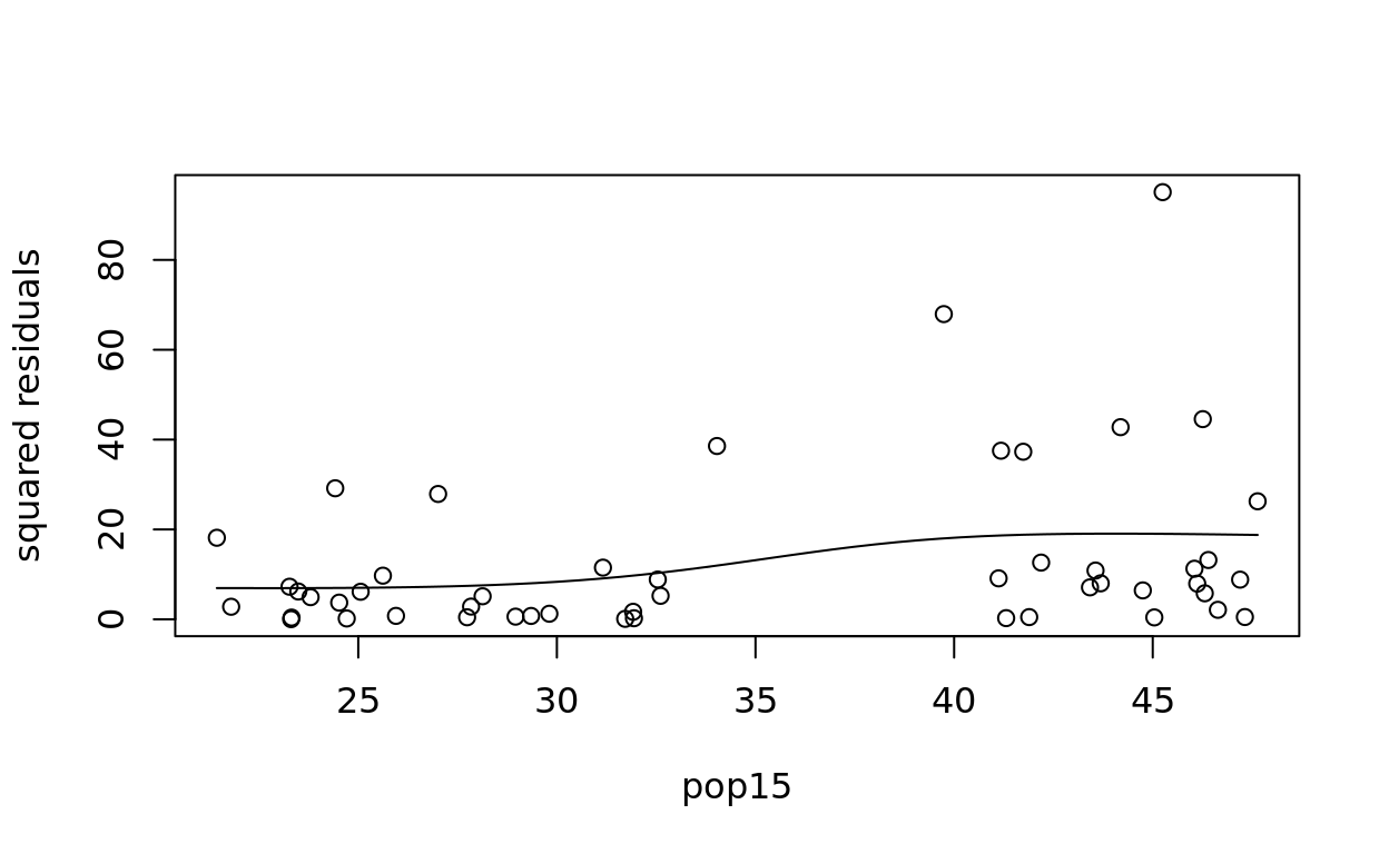
#We will use 1/fitted(var) as the weight variable in an lm to downweight cases with large predicted squared variance
#as related to pop15.
g.wls = lm(sr ~ pop15+pop75+dpi+ddpi,savings, weights=1/fitted(var1))
plot(pop15, sr)
abline(g)
abline(g.wls,lty="dashed",col='red') #See how the wls line is gravitating less toward the high sr cases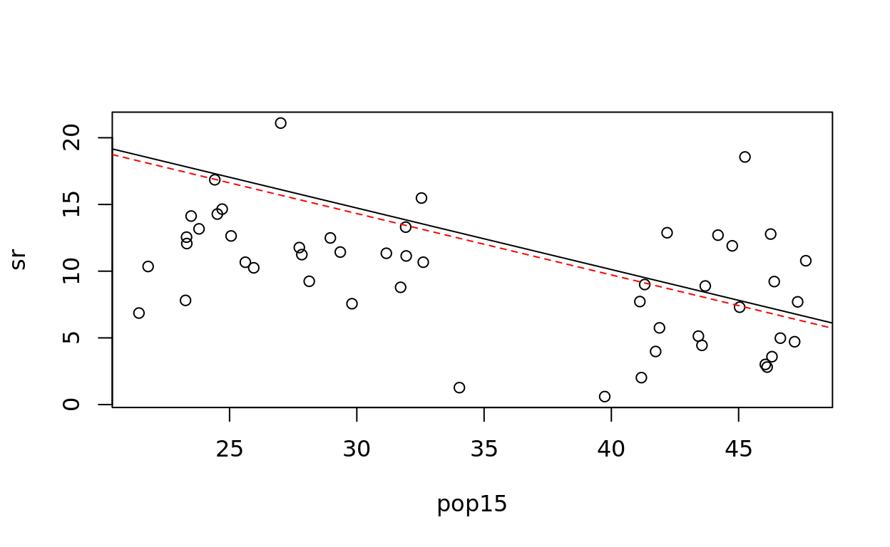
Let’s check the squared residuals again.
plot(pop15, residuals(g)^2,ylab="squared residuals") #Looks like there is a strong relation there!
points(pop15, residuals(g.wls),pch=15, col="red")
var.wls = npreg(residuals(g.wls)^2 ~ pop15)
##
Multistart 1 of 1 |
Multistart 1 of 1 |
Multistart 1 of 1 |
Multistart 1 of 1 /
Multistart 1 of 1 |
Multistart 1 of 1 |
lines(grid.x, predict(var1, exdat=grid.x))
lines(grid.x, predict(var.wls, exdat=grid.x),lty="dashed",col="red")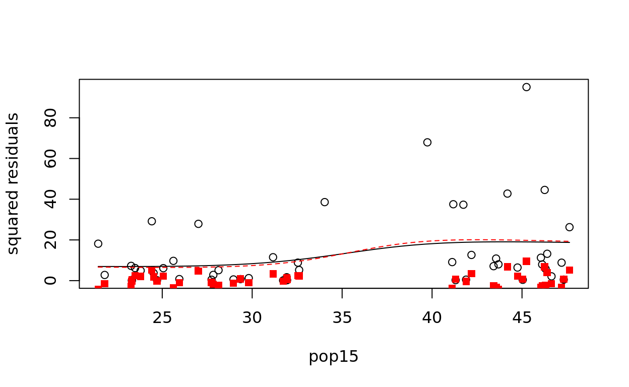
summary(g)##
## Call:
## lm(formula = sr ~ pop15 + pop75 + dpi + ddpi, data = savings)
##
## Residuals:
## Min 1Q Median 3Q Max
## -8.2422 -2.6857 -0.2488 2.4280 9.7509
##
## Coefficients:
## Estimate Std. Error t value Pr(>|t|)
## (Intercept) 28.5660865 7.3545161 3.884 0.000334 ***
## pop15 -0.4611931 0.1446422 -3.189 0.002603 **
## pop75 -1.6914977 1.0835989 -1.561 0.125530
## dpi -0.0003369 0.0009311 -0.362 0.719173
## ddpi 0.4096949 0.1961971 2.088 0.042471 *
## ---
## Signif. codes: 0 '***' 0.001 '**' 0.01 '*' 0.05 '.' 0.1 ' ' 1
##
## Residual standard error: 3.803 on 45 degrees of freedom
## Multiple R-squared: 0.3385, Adjusted R-squared: 0.2797
## F-statistic: 5.756 on 4 and 45 DF, p-value: 0.0007904summary(g.wls)##
## Call:
## lm(formula = sr ~ pop15 + pop75 + dpi + ddpi, data = savings,
## weights = 1/fitted(var1))
##
## Weighted Residuals:
## Min 1Q Median 3Q Max
## -1.92871 -0.71075 -0.08478 0.74133 2.19172
##
## Coefficients:
## Estimate Std. Error t value Pr(>|t|)
## (Intercept) 28.1194603 6.2967726 4.466 5.32e-05 ***
## pop15 -0.4600341 0.1253273 -3.671 0.000639 ***
## pop75 -1.6381814 0.8897586 -1.841 0.072197 .
## dpi -0.0003658 0.0007413 -0.494 0.624056
## ddpi 0.5187820 0.2011923 2.579 0.013264 *
## ---
## Signif. codes: 0 '***' 0.001 '**' 0.01 '*' 0.05 '.' 0.1 ' ' 1
##
## Residual standard error: 1.033 on 45 degrees of freedom
## Multiple R-squared: 0.4023, Adjusted R-squared: 0.3492
## F-statistic: 7.574 on 4 and 45 DF, p-value: 9.384e-05We see that our conclusions stay exactly the same. That is good! That shows that our results are pretty robust to changes in the homoscedasticity assumption.
Solutions
avPlot(g,variable="ddpi")# Specify g.IV as a model in which ddpi (the "added IV") is predicted using all other IVs
g.IV = lm(ddpi ~ pop15+pop75+dpi,savings)
# Get the residuals
resid_ddpi = residuals(g.IV)
# Now specify g.DVnoddpi as a model in which the DV (sr) is predicted using all other IVs but ddpi
g.DVnoddpi = lm(sr ~ pop15+pop75+dpi,savings)
#Get the residuals from the model with no ddpi
residsr_noddpi = residuals(g.DVnoddpi) qqnorm(residuals(g),ylab="Residuals")
qqline(residuals(g))
#qqPlot function from the car library
qqPlot(residuals(g), main="qqPlot function from car")
shapiro.test(residuals(g))